Aggregation and Disaggregation
What is (Dis)Aggregation?
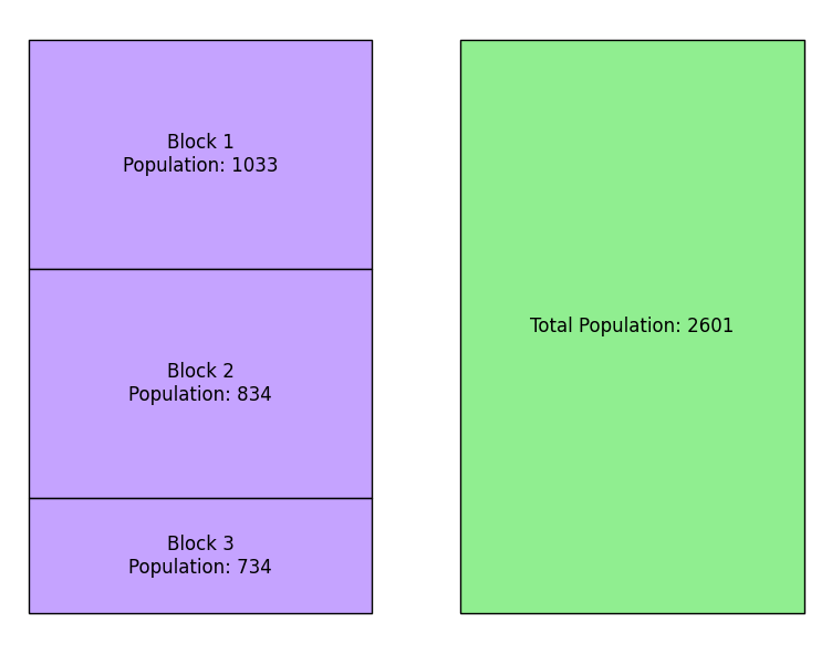
Aggregation is the process of grouping observations together to calculate summary data for some larger area. For example, one could sum the total population in 3 adjacent census blocks to report the total population of a particular area, as shown in the figure below.
Aggregating the Population in 3 Census Blocks
Disaggregation is the reverse process of breaking down aggregated data into smaller units. Disaggregated data will always be an estimate, as is the case for disaggregating election results from precincts to census blocks.
In both aggregation and disaggregation, the geographic unit for which data is known is often referred to as the source, while the geographic unit for which data is desired and unknown is referred to as the target.
Why Aggregate and Disaggregate?
In redistricting, data is often needed at levels of geography that it is not reported at. For example, data may be desired at the district level, but census data is frequently reported at geographies such as block groups or census tracts, while election data is typically reported at the precinct level.
Because these geographies intersect in ways that make it difficult to directly aggregate the data, it is necessary to first disaggregate election results (usually at the precinct level) or demographic data (usually at the block group or tract level) to the smallest unit possible: the census block level. Since state legislative and congressional districts – and many other census geographies – are formed out of census blocks, the data can then be aggregated up to the district level.
Another common situation that calls for aggregation and disaggregation is when trying to analyze demographic and election data simultaneously, as in the case of racially polarized voting analyses. Census data is available on census blocks (or other census geographies), which are typically smaller and sometimes split the precinct geographies at which election results are reported. As a result, block level census data must be aggregated to precincts or precinct level election data disaggregated to blocks, to analyze both kinds of data simultaneously.
The Role of Spatial Data in Assignment
In order to (dis)aggregate, target geographies must be mapped, or assigned, to source geographies. This process can be spatial or non-spatial in nature.
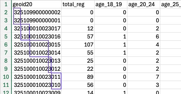
In non-spatial assignment, the relationship of the target geographies to the source geographies is known in advance. For example, the Census Bureau has devised a clear system in which census blocks nest neatly within block groups, block groups nest neatly within census tracts, census tracts nest neatly within counties, and counties nest neatly within states. This assignment is identified by “geoid” values. Because it is known which blocks nest in which block groups (and so on), no geospatial data is required to aggregate or disaggregate these census geographies.
Non-Spatial Assignment with Census Data
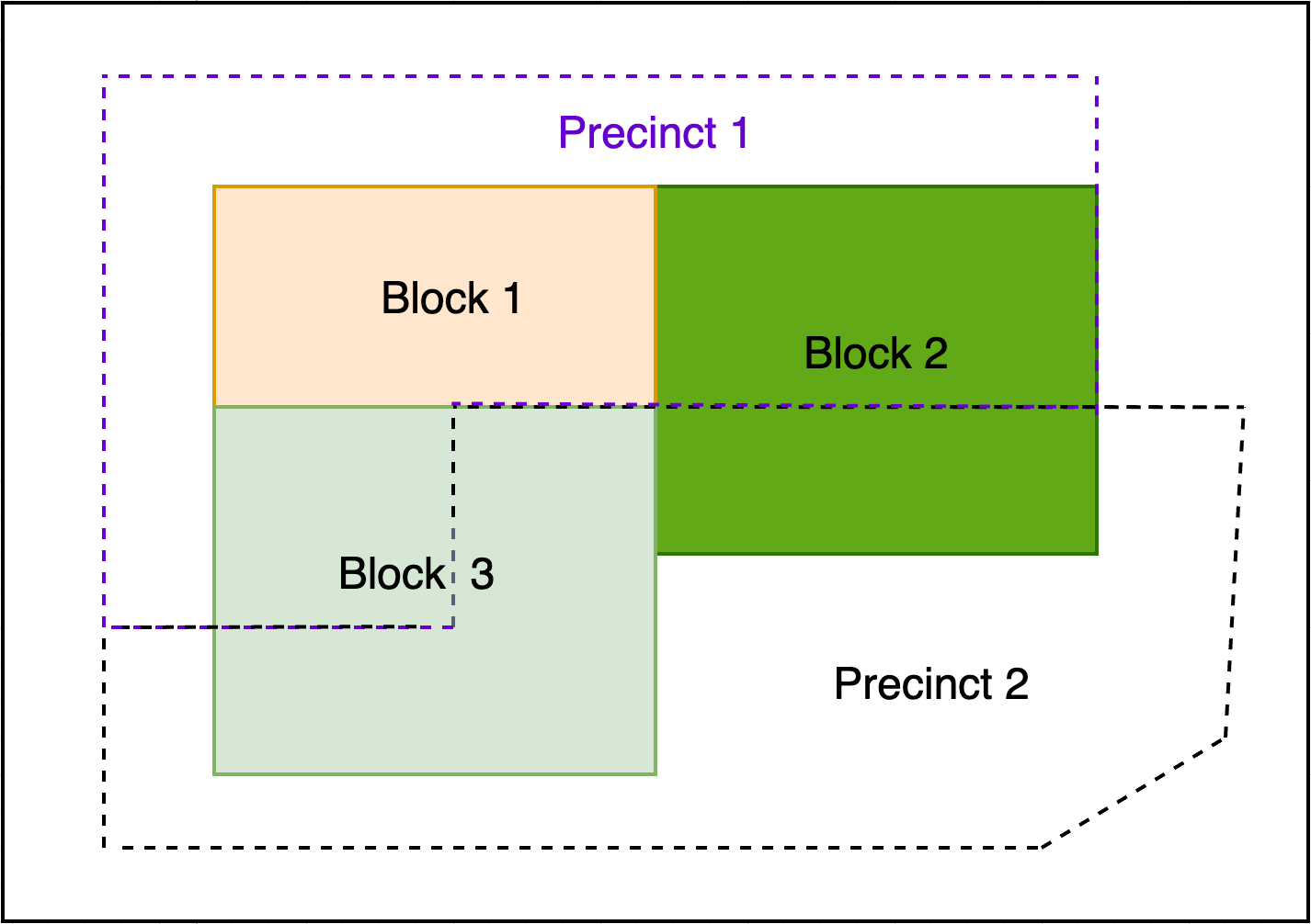
In spatial assignment, the relationship of the target geographies to the source geographies is not known in advance and must be found using spatial data. This is often the case when working with precinct level election results and demographic data on census blocks. To aggregate block level data to precincts, for example, the exact boundaries of these precincts must be known and mapped against the block boundaries, in order to appropriately assign blocks and create the best estimated aggregation of the data at the precinct level.
Some states work hard to align census blocks with precincts, making the mapping of source to target geographies relatively straightforward. Other states do not, however, and many precincts may be split. There is also a great deal of variation in the degree or “seriousness” of the split – some precincts may split blocks ever so slightly, and is more likely a function of data quality rather than purposeful misalignment.
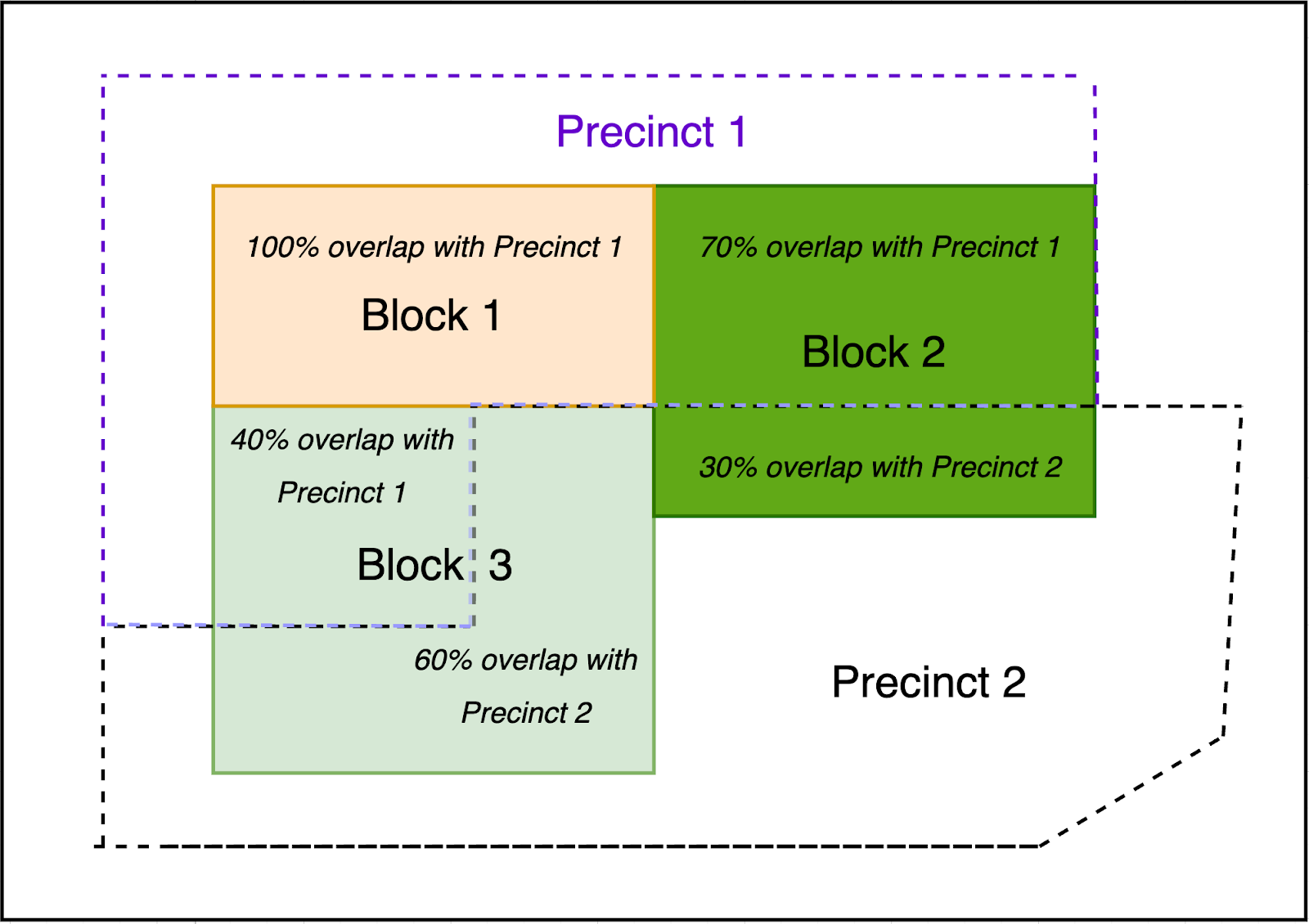
Spatial Assignment of 3 Census Blocks to 2 Precincts
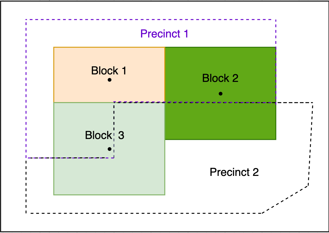
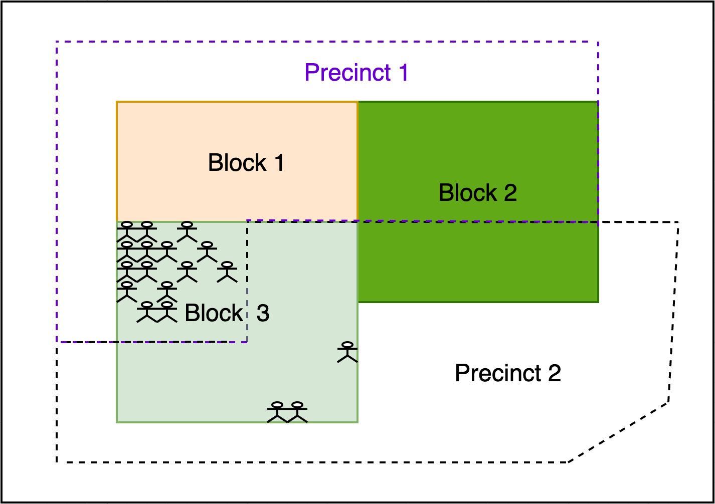
One way to assign source geographies to target geographies is to use the source’s geographic center point, known as the centroid. For example, if the centroid of a census block falls in a particular precinct, then that block will be assigned to the precinct.
Spatially Assigning Census Blocks to Precincts Based on Centroids
Another method is to assign sources to target geographies based on the largest amount of areal overlap. If 60% of a block overlapped with a precinct and the remaining 40% with another, we would assign the block to the precinct with which it shares 60% of the same geography. This is the default method taken by the Python package maup, created by our Data Partner the Metric Geometry and Gerrymandering Group.
Spatially Assigning Census Blocks to Precincts Based on Areal Overlap
How to Aggregate or Disaggregate
In addition to assignment, additional information is needed about the target geographies to estimate how the aggregated source data should be distributed and disaggregated. The more accurately the information at the target geography represents what you are trying to disaggregate, the better the disaggregation will be.
Mathematically, disaggregation is the process of solving for an equation where two ratios are equal to one another, and you are trying to solve for X1:
Block Level Data Y1 (known) Block Group Level Data Y2 (known) = Block Level Data X1 (unknown) Block Group Level Data X2 (known)
For example, the Census Bureau releases citizen voting age population (CVAP) data, but only at the block group level. We can use the 2020 PL 94-171 census data at the block level, which provides counts of the total population, total population by race/ethnicity, total voting age population (VAP, or the population 18 and over), and VAP by race/ethnicity to disaggregate the CVAP data.
Specifically, the RDH team uses counts of the population by race/ethnicity according to the 1997 OMB categories to disaggregate the block group estimates of CVAP by race/ethnicity. We calculate the ratio of each block’s VAP (by race/ethnicity) relative to each block group’s CVAP (by race/ethnicity), and multiply the block group’s population by that ratio to estimate the population in each block, using the equation above.
To disaggregate election results, the RDH team uses a modified VAP, which subtracts the adult (18 years and older) incarcerated population reported in the P5 table of the 2020 PL 94-171 decennial census data from the total VAP.
There are many possible disaggregators, and what is most appropriate depends on a given dataset. For example, the RDH team has used data on the number of households (for disaggregating household data) and the 25 years and older population (for disaggregating educational attainment). It is also possible to disaggregate data based on a combination of factors: for example, if VAP from the decennial census is the desired disaggregator, but the data to be disaggregated is from the middle of the decade (say, 2015), one could use an average of the 2010 and 2020 VAP data.
It is important to understand that disaggregated data will often result in fractional values. For example, if a precinct had 3 votes that were disaggregated into two census blocks, one might end up with 1.5 votes in each. Of course, there is no such thing as a half of a vote. As such, rounding these values is appealing, so that the vote totals “make sense.” But if one were to blindly round using the usual method (anything .5 and above rounds up, anything .49 and below rounds down), it is easy to distort the totals. In our simple example, 1.5 would get rounded up to 2, resulting in 4 votes at the census block level, whereas only 3 votes were cast at the precinct level. Fortunately, other rounding methods exist that avoid these kinds of distortions, such as the Hamilton method, which the RDH team uses, or the method of largest remainders.
For more details on the process, see our Python code for election disaggregation. Disaggregation code for various datasets can also be found on our Github page.
Assumptions in (Dis)Aggregation and Assignment
Depending on whether one is aggregating or disaggregating data, and whether one is doing spatial or non-spatial assignment, one or more assumptions may be involved in the process.
When aggregating data non-spatially, likely no assumptions are involved. For example, aggregating census data from blocks to block groups requires no assumptions, as it is simply a matter of summing up data across source geographies to calculate the data for the target geography.
If the aggregation is spatial in nature, however, then one assumes the method of assigning source to target geographies is correct. For example, if one were to aggregate data on the total population from blocks to precincts by largest areal overlap, one assumes that all the people in those blocks should be assigned to and counted in a particular precinct.
In redistricting, the question of interest is typically focused on people, or voters. Ideally, the spatial distribution of people in a block would determine whether to assign source to target geographies based on the centroid, areal overlap, or something else.
However, such sub-block data is rarely available. Key demographic data from the Census Bureau is only available at the census block level or above, and it is unknown precisely where people live within a block. Address data for voters is available in voter registration files, but these can be prohibitively expensive to purchase in some states. Regardless of the cost, this approach would require extensive work to first geocode voters, then cross-reference their addresses with census blocks, and finally determine the proportion of each block’s population that lives in each precinct.
The Method of Spatial Assignment as an Assumption
The assumption of correct assignment is required whether aggregating or disaggregating data. But there is a second set of assumptions that is made when disaggregating data specifically, and that is that a) the choice of the disaggregator is correct, and b) the relationship between the two ratios is correct.
A good example can be made from using education data. If a state released county level data on the total population with bachelor degrees (BAs/BSs), one might be interested in disaggregating that data to census tracts. The Census Bureau has educational data at the census tract level, but only for people 25 years of age and older. As a result, one might establish the following equation to solve for X (the population with bachelor degrees at the census tract level):
Census Tract Population 25+ with Bachelor Degrees County Population 25+ with Bachelor Degrees = X County Population with Bachelor Degrees
This equation assumes that the ratio between the county and census tract populations 25 years of age and older, and the ratio between county and census tract populations with a bachelor degree, are equal to one another, and that the choice to use the census tract population 25 and over with a bachelor degree is the correct disaggregator. Ultimately, these assumptions may be correct in certain situations and incorrect in others.
Validation
We check our aggregation and disaggregation by summing up the totals of the (dis)aggregated geographies to ensure they match the original summed values. If there are holes or overlaps across the source and target geographies, the assignment process can break down and data can be lost. As a result, it is very important to ensure that all data is retained during the (dis)aggregation process. Once this is confirmed, we are now able to analyze this data, or join it with other datasets available at the same unit of geography.
Questions about (dis)aggregation?
Our help desk team is here to help.
Send a message and they will respond within one business day!